As a beginner of deep learning, it’s quite easy to get lost when you attempt to compute the gradient on a recurrent neural network(RNN). Therefore, we will give the computation of gradients on RNN by backforward propagation through time(BPTT). I assume that you have known the concept of backward-propagation algorithm, recurrent neural networks(RNN), linear algebra and matrix calculus before the exploration.
Notations
These notations used in the following computation refer to the book Deep Learning.
$
\begin{array}{l|l}\hline
a & \text{Scalar a}\\\hline
\boldsymbol{x} & \text{Vector x} \\\hline
\boldsymbol{1}_{n} & \text{A vector [1,1,…,1] with n column}\\\hline
\boldsymbol{A} & \text{Matrix A}\\\hline
\boldsymbol{A}^{-1} & \text{The inverse matrix of matrix A}\\\hline
\boldsymbol{A}^{\mathsf{T}} & \text{Transpose of matrix A}\\\hline
\text{diag}(\boldsymbol{a}) & \text{Diagnal matrix with diagnal entries gieven by }\boldsymbol{a}\\\hline
\boldsymbol{I} & \text{Identity matrix}\\\hline
\nabla_{\boldsymbol{x}}y & \text{Gradient }y\text{ with respect to }\boldsymbol{x} \\\hline
\frac{\partial{y}}{\partial{x}} & \text{Partial derivative of } y \text{ with respect to }x\\\hline
\frac{\partial{\boldsymbol{y}}}{\partial{\boldsymbol{x}}} & \text{Jacobian matrix }\boldsymbol{J} \in \mathbb{R}^{m \times n} \text{of } f:\mathbb{R}^{n}\to\mathbb{R}^{m} \\\hline
\end{array}
$
Review of RNN
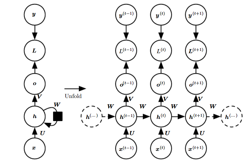
Figure 2.1: The computational graph of RNN @Deep Leaerning
Let’s develop the forward propagation equations for the RNN dipcted in Figure 2.1. As a convenience, we use right superscription to indiacte the specified state of RNN at some time $ t $.
To represent the hidden units of the network, we use the variable $ \boldsymbol{h} $, which will be the input of hyperbolic tangent activation function. As you see, the RNN has input-to-hidden connections parametrized by a weight matrix $ \boldsymbol{U} $, hidden-to-hidden connections parametrized by a weight matrix $ \boldsymbol{W} $, hidden-to-output connections parametrized by a weight matrix $ \boldsymbol{V} $. We can apply the softmax operation to the output $ \boldsymbol{o} $ to obtain a vector $ \boldsymbol{\hat{y}} $ of normalized probabilities over the output. We define the loss function as the negative log-likelihood of output vector $ \boldsymbol{\hat{y}} $ given the training target $ \boldsymbol{y} $. With notations and definitions made, we have the following equations:
where both $ \text{tanh} $ and $\text{log}$ are element-wise function.
Taking the Derivatives
Known the notations and concepts above, we can compute the gradients by BPTT using the identities below.
| Conditions | Expression | Denominator layout |
|---|---|---|
| $ \boldsymbol{A} $ is not a function of $ \boldsymbol{x} $ | $ \frac{\partial{\boldsymbol{Ax}}}{\partial{\boldsymbol{x}}} $ | $ \boldsymbol{A}^{\mathsf{T}} $ |
| $g(\boldsymbol{U})\text{ is a scalar, }\boldsymbol{U} = \boldsymbol{U}(\boldsymbol{X}) $ | $\frac{\partial{g(\boldsymbol{U})}}{\partial{\boldsymbol{X}}_{ij}} $ | $\text{tr}\left(\left(\frac{\partial{g(\boldsymbol{U})}}{\partial{\boldsymbol{U}}}\right)^{\mathsf{T}}\frac{\partial{\boldsymbol{U}}}{\partial{\boldsymbol{X}}_{ij}}\right) $ |
we here will give three examples of computations in detail.
Example 1
To begin with, we will take the derivative of loss function $ L $ with respect to vector $ \boldsymbol{o} $. Using denominator-layout and chain rule, we have:
Taking the former derivative of $ \boldsymbol{\hat{y}} $ with respect to $ \boldsymbol{o} $, we get:
For the latter partial derivative, we have:
Therefore, gradient $ \nabla_{\boldsymbol{o}^{(t)}}L $ at time step $ t $ is as follows:
where the training target $ \boldsymbol{y} $ is a basic vector [0,…,0,1,0,…,0] with a 1 at the postion $ i $.
Example 2
Now, we consider a slightly more complicate example: computation of $\nabla_{\boldsymbol{h}^{(t)}}L$.
Walking through computational graph backforward, it’s easy to get the gradient at the final time step $ \tau $ because the $\boldsymbol{h}^{(t)}$ has only a descendent $\boldsymbol{o}^{(t)}$:
However, we should note that the $\boldsymbol{h}^{(t)}$ has both $\boldsymbol{o}^{(t)}$ and $\boldsymbol{h}^{(t+1)}$ as descendents from $ t = \tau - 1 $ down to $t = 1$. Consequently, the gradient is given by:
Taking the two cases above into account, we have:
Example 3
Once the gradients on internal nodes were computed, we can take the derivatives of the parameters, e.g. $ \boldsymbol{W} $, $ \boldsymbol{V} $. Notice that the parameters are shared across the time steps, we will introduce some dummy variables such as $\boldsymbol{W}^{(t)}$ that are define to be copies of parameter but with each only used at time step $t$, which will be accumulated from $ t = \tau $ down to $ t = 0 $ so that we can obtain the gradient $ \nabla_{\boldsymbol{W}}L $ at the end of a backward propagation.
Applying the notations above, the gradient on the parameter $\nabla_{\boldsymbol{V}}L $ is given by:
In fact, inspired by the relationship between total derivative and partial derivative in multivariable calculus:
which can be written in vector form as:
we can obtian the relationship between total derivative and partial derivative in matrix calcalus:
Now, we can skip the tedious process (3.3.1) by applying eq. (3.3.4) for gradient $ \nabla_{\boldsymbol{V}}L $:
We could derive the result by comparing eq. (3.3.4) with eq. (3.3.5):
Similarly, using the equation (3.3.4), the gradient on remaining parameters is quite easy to get and we can gather these gradients as follows: